Brownian Motion: the Drunken Amnesiac Particle

UPDATE: Luke Palmer helped me fix the problem, and now the distribution looks uniform!
The above rendering is with the new code, which replaced the old code below.

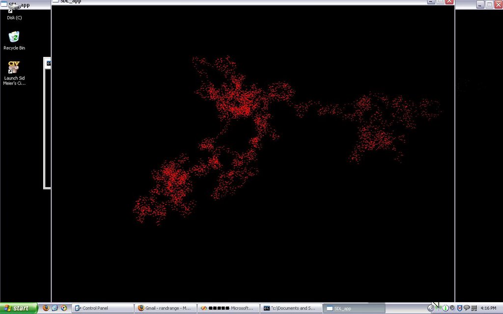
We learned about Brownian motion in fractal class today, so I programmed up a little guy to run around drunkenly, and I taught him to drop breadcrumbs so that I could see where he went. The result is quite beautiful, even though the fundamental basis of the rendering is totally "random," meaning the directions of the steps are taken from a random seed.

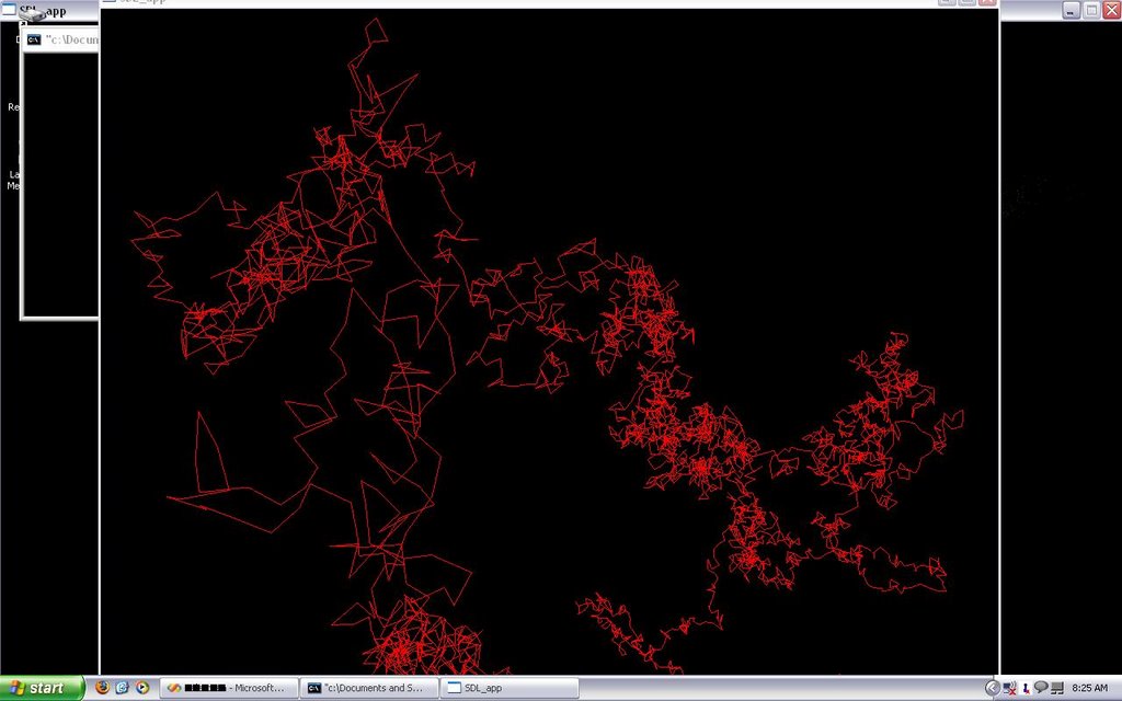*UPDATE*: I was falling asleep last night, when the thought struck me that I should show the path of the particle as opposed to a cloud of points. It seems so *$%#&ing obvious to me now that I can't imagine how I didnt think of it this way to begin with. After I implemented the path trace (see above rendering), I thought back to my CAGD class (Computer-Aided Geometric Design) and remembered b-splines. The idea of a b-spline is to extend a Bezier curve into a long "frankenstein" curve that is a concatenation (and combination) of any number of Bezier curves into one composite curve, which is defined by the control points and a sequence of knots which define the time spent in each portion of the curve (which basically means "how fast the particle is moving through the various sections of the curve"). This technique is used extensively in computer animation, for example Pixar films. The animators use a b-spline to trace the path of an object through the virtual world, like a ufo flying through space, and the knot sequence determines the acceleration and speed of the ship through the various turns, twists, and straights.

If I have some time, and if I can get my head around it, I will try to turn the path of the particle into a sequence of control points for a b-spline. The knot sequence wouldnt be too important for this application, but to ensure that the curve is as smooth as possible, they should be uniformely spaced through the middle, one per control point, and a multiplicity of two or three on the endpoints. The end result of this method would be a nice, pretty, smooth curve that represented the particle's path as opposed to the sharp, geometric, computerized form that it has currently.

Also, I think that it would be a closer approximation of actual brownian motion, because I would be treating my collection of points as a sample instead of a population. The b-spline would approximate what the particles actual path might have been, since in reality the particle's path would be continuous (at least) through its second derivative (not sure about this... any math people want to comment or correct me or give a specific explanation?). If I used the b-spline technique, it would be C2 and G2 continuous, which mean, *basically* (look them up for more detailed info), that the curve is continuous on its first and second derivatives through all junctions.

*END UPDATE*

************2ND UPDATE*****************

Brownian Motion in full continuous glory! I used the path samples as control points and formed a uniform cubic b-spline! Now the particle appears to actually fly through the air in a somewhat realistic way. The laws of physics are no longer put on hold!

Here is the equation that I used for you b-spline junkies:

vec result= (1.0f/6.0f) * (pow((1-t), 3) * p[3] + (3 * pow(t, 3) - 6 * pow(t, 2) + 4) * p[2] + (-3 * pow(t, 3) + 3 * pow(t, 2) + 3 * t+1) * p[1] + pow(t, 3) * p[0]);

Where p[0], p[1], p[2], p[3] are current and previous 3 points. p[0] is the current point, p[1] is i-1, and so forth, and t is a parameter that ranges across [0, 1] by increments. In these renderings, I used an increment of 0.05 to get 20 piecewise chunks for each curve segment. As t goes from 0->1, the curve from p[1] to p[0] is traced using the information of the previous points to maintain continuity.

This is a very basic b-spline equation but it does the trick. If you want to see a more palatable (but less functional) representation of this equation, go to wikipedia and search for "cubic b-splines" or just "b-splines."

Here are some renderings: DONT CLICK ON THEM FOR A CLOSER LOOK! because of the smoothness of the curve, there are some major aliasing problems resulting from blogger's compression. The best way to view these renderings is the way they look here on the page.

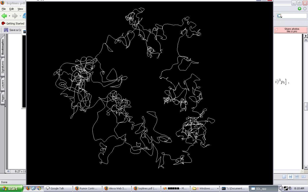
note: although it appears that there are some cusps, keep in mind that these are fully 3d particle path traces, and if viewed from a different angle, the cusps are all revealed to be tight loops.

***********end 2ND UPDATE********************




The code I am posting should be completely executable (if you set up an opengl window), and providing you write a function called randrange(float min, float max), which returns a random floating point number between the two boundaries.

Note: I still cant post code properly for some reason, even when i use the tags that they say should work online. I have changed the line that keeps getting chopped out with psuedocode. This is the best solution i could come up with. sorry.

[code]
class brown
{
public:
vec position;//mean

float range; //"variance"

int stepcount;

bool live;

vec varray[2000000];
int varray_cursor;

brown()
{
position=vec();//(0,0,0)
range=100;
stepcount=0;
live=true;

varray_cursor=0;

srand(time(NULL));
}


float randrange(float min, float max)
{
return float(rand()) / RAND_MAX * (max - min) + min;
}


step()
{
vec direction;

direction.x=randrange(-1, 1);
direction.y=randrange(-1, 1);
direction.z=randrange(-1, 1);

direction=(~direction)/10.0f;

int count=1;
//pseudocode
for(int i=0; i less than range; i++)
//end pseudocode
{
if(((int)randrange(0, 1000))%2==0)
count++;
}

direction*=count;

position+=direction;


varray[varray_cursor].x=position.x;
varray[varray_cursor].y=position.y;
varray[varray_cursor].z=position.z;
varray[varray_cursor+1].x=position.x;
varray[varray_cursor+1].y=position.y;
varray[varray_cursor+1].z=position.z+2.0f;
varray_cursor+=2;
}

tick()
{
if(live)
step();
if(stepcount>=1000000)
live=false;

draw();
}


void draw()
{
glColor3f(1, 0, 0);
glEnableClientState(GL_VERTEX_ARRAY);

glVertexPointer(3, GL_FLOAT, sizeof(vec), &varray[0].x);
glDrawArrays(GL_LINES, 0, varray_cursor*2);
}

};

[/code]

By changing the variable "prob", the "width" of the drunken particle's path is increased or decreased, which accounts for the difference between the crack above and the nebulous cloud below. The closer prob is to -1, the thicker the cloud. The closer prob is to 1, the narrower the cloud. (note: the code no longer works this way. Luke pointed out that there is an inherent bias towards the negative in computer representations of numbers, so the code has been changed to a x%2=0 binary selection where x is a random number. The steps can be as long as 100, but it is insanely unlikely. This represents a somewhat reasonable probability structure, but not a bell curve. This is more like a gravity well than a bell curve.)



Clearly something is broken here. I would expect the particle to wander more aimlessly than it does. It seems as if either x, y, or z is biased towards a single direction. It is not completely locked in that direction, as can be seen if you watch the particle in motion (which will go in seemingly random directions on a local scale), but there is a definite large scale trend as if the particle is actually trying to get somewhere, despite constantly forgetting where it is and where it came from.

(This is no longer broken, as can be seen at the top of the post. It looked interesting when it was broken anyway, though, so it stays up).